Building a Air Quality Forecasting Pipeline with a Feature Store

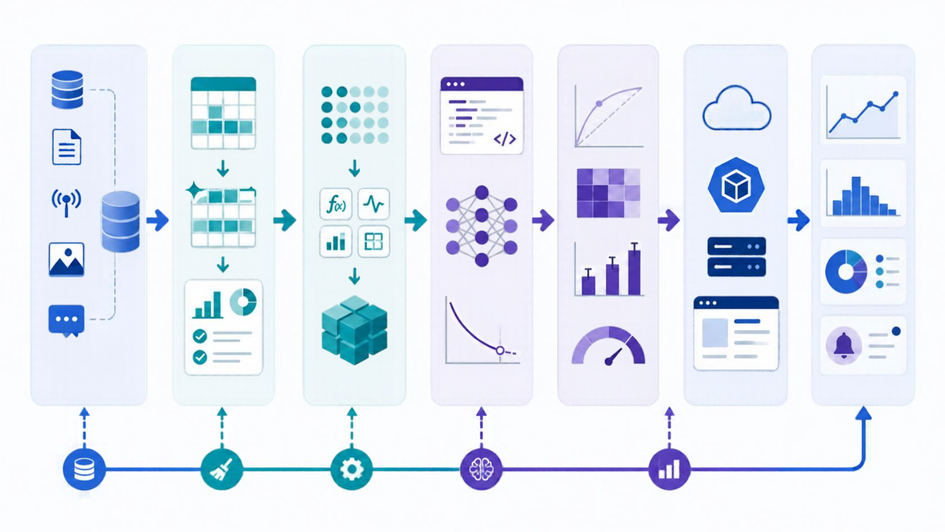
In this blog, we will use a real example to demonstrate how MLOps can be implemented using GitHub Actions. While this example highlights the importance of MLOps, please note that we are not deploying in a production environment. For production deployment, we would require robust tools and deployment options.
Air quality affects everyone, but most public dashboards only tell you what the air was like today. I wanted to know what it would be like a week from now, so I built a small end-to-end ML system that forecasts PM2.5 (fine particulate matter) for my city, running entirely on free-tier infrastructure with no servers to manage.
This post walks through the architecture, the data, the model, and where it's headed next.

The Goal

Predict PM2.5 concentration for the next 7 days for a single location (Greensboro, NC in my case), refresh the forecast daily, and publish it as a public dashboard — without running any infrastructure myself.

Why a Feature Store?

The classic failure mode in small ML projects is "notebook spaghetti": one notebook pulls data, transforms it, trains a model, and makes predictions, all in one place, with no clean separation between the parts that change daily (new data) and the parts that change occasionally (model training). That makes it hard to reason about, hard to monitor, and hard to debug when a forecast looks wrong.

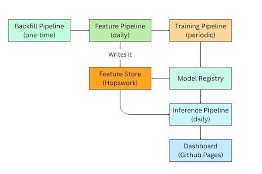
Instead, I split the system into four independent pipelines connected through a feature store (Hopsworks):

1. Backfill Pipeline — one-time load of historical PM2.5 readings and historical weather, to give the model years of training data.

2. Feature Pipeline — runs daily, fetches today's PM2.5 reading and weather forecast, validates it, and writes it to the feature store.

3. Training Pipeline — trains an XGBoost regressor on the accumulated feature history. Run manually / periodically, not daily.

4. Inference Pipeline — runs daily, pulls the latest model and the weather forecast features, and produces a 7-day PM2.5 forecast.

Each pipeline is a Jupyter notebook, executed non-interactively with jupyter execute (originally designed for Papermill) inside a GitHub Actions workflow. This keeps the project serverless: there's no always-on compute, just scheduled jobs that spin up, do their work, and shut down.

Data Sources

Two public, free APIs feed the system:

• World Air Quality Index (WAQI) — real-time PM2.5 readings from a physical sensor near my location.

• Open-Meteo — historical weather (temperature, precipitation, wind speed, wind direction) for training, and ECMWF-based weather forecasts for the days we want to predict air quality for.

The core modeling assumption is that weather conditions — wind, rain, temperature — are strong drivers of local particulate concentration, so forecasted weather can be used as a proxy feature set to forecast future PM2.5.

Feature Store + Data Validation

Every row written to the feature store passes through Great Expectations validation first — for example, asserting that pm25 falls within [-0.1, 500] and that wind speed is non-negative. This catches bad sensor readings or malformed API responses before they can silently corrupt the training data, which matters a lot more once a pipeline is unattended and running on a daily cron.

Two feature groups exist in the store:

• air_quality — date, PM2.5 reading, location metadata.

• weather — date, temperature, precipitation, wind speed, wind direction.

A feature view joins them on date/city, with pm25 as the label and the four weather variables as features — intentionally small and interpretable.

The Model

The current approach utilizes an XGBRegressor, which is an advanced and highly efficient machine learning model specifically designed for regression tasks. This model is part of the XGBoost library, known for its scalability and speed. The XGBRegressor is particularly effective due to its implementation of gradient boosting, which optimizes the model's performance by combining the predictions from multiple weak learners to produce a strong final prediction. This makes it well-suited for handling large datasets and addressing various complexities in the data, resulting in more accurate and reliable outcomes.

The training data consists of a substantial dataset, encompassing approximately 3,500 days of historical records that combine weather conditions—such as temperature, humidity, and precipitation—with corresponding PM2.5 levels, a critical indicator of air quality. This extensive dataset provides a rich context for understanding how weather patterns influence pollution levels over time.

For the model evaluation, we adopt a time-based test set strategy, specifically holding out the last 30 days of data. This method is vital for time series analysis, as it respects the chronological order of observations, preventing any potential leakage of future information into the training phase. By avoiding random splits, which could mislead the model by allowing it to train on data that it should not have access to during testing, we ensure a more accurate assessment of the model's predictive capabilities in a real-world scenario. This careful design enhances the integrity of the evaluation process, ensuring that the results reflect the model's true performance when forecasting future PM2.5 levels based on weather data.

xgb_regressor = XGBRegressor()
xgb_regressor.fit(X_train[['temperature_2m_mean', 'precipitation_sum',
                            'wind_speed_10m_max', 'wind_direction_10m_dominant']],
                   y_train)

The trained model, along with its metrics, is versioned in the Hopsworks Model Registry — so the daily inference pipeline always pulls a known, reproducible model artifact rather than retraining from scratch every day.

Where It Stands, and What's Next

The current model is intentionally minimal: four same-day weather features and default XGBoost hyperparameters. It's a baseline, not a finished product, and there's a clear roadmap to improve it:

• Lag and rolling-window features — yesterday's PM2.5, a 3-day rolling average. Air quality tends to be autocorrelated day-to-day, so this is likely the single highest-leverage addition.

• Seasonality features — day-of-year, month, since pollution patterns shift with seasons (heating season, wildfire season, etc.).

• Hyperparameter tuning — max_depth, n_estimators, learning_rate via time-series cross-validation instead of defaults.

• A naive persistence baseline ("predict same as yesterday") to make sure any added model complexity is actually earning its keep.

• Additional sensors — spatial signal from neighboring stations could help triangulate pollution sources.

Monitoring: Hindcasting

Rather than trusting the offline test metrics forever, the inference pipeline also writes a hindcast: every day, it compares the prediction made 1 day ago against the actual outcome that arrived today, and stores both in a dedicated aq_predictions feature group keyed by (city, street, date, days_before_forecast_day). This produces a live, continuously-updating accuracy chart rather than a one-time offline number — which is the number that actually matters once a model is in production.

monitoring_df = monitor_fg.filter(monitor_fg.days_before_forecast_day == 1).read()
hindcast_df = pd.merge(monitoring_df, air_quality_df[['date', 'pm25']], on='date')

Automation

A single GitHub Actions workflow (.github/workflows/blank.yml) ties it together, running daily at 6:11 AM UTC:

on:
  workflow_dispatch:
  schedule:
    - cron: '11 6 * * *'

steps:
  - run: |
      cd notebooks
      jupyter execute feature_pipeline.ipynb
      jupyter execute batch_inference.ipynb
  - uses: stefanzweifel/git-auto-commit-action@v7
    with:
      commit_message: "Air Quality Dashboard published"
      file_pattern: 'docs/air-quality/img/*'

The feature pipeline ingests today's sensor reading and forecast weather; the inference pipeline generates the forecast and hindcast charts as PNGs; the auto-commit action pushes the updated images straight into docs/, which GitHub Pages serves as a static dashboard. No server, no cron daemon to babysit, no deployment step beyond git push.

MLOps in Practice

It's easy to treat "MLOps" as an abstract buzzword. Concretely, in this project it shows up as five specific engineering decisions:

1. Pipeline decomposition (CI/CT/CD for ML). Instead of one notebook that does everything, the system is split into pipelines with different trigger cadences — feature and inference run daily, training runs on demand, backfill runs once. This is the ML analogue of separating build/test/deploy in traditional CI/CD: each stage has a single responsibility and can be triggered, scaled, or debugged independently. GitHub Actions is the orchestrator, standing in for tools like Airflow or Kubeflow Pipelines at a much smaller scale.

2. Feature store as the contract between pipelines. The feature and training/inference pipelines never talk to each other directly — they only read and write through Hopsworks. That decouples "how data is produced" from "how it's consumed," and guarantees training and serving use identically-computed features (avoiding training/serving skew, a classic source of silent ML bugs).

3. Model registry for versioning and reproducibility. The trained model isn't a loose model.json file passed around by hand — it's registered in Hopsworks' Model Registry along with the metrics (MSE, R², sample counts) it was trained and evaluated with, and the feature view it depends on. The inference pipeline always fetches a specific registered version, so "which model produced this forecast" is always answerable, and retraining never silently overwrites history.

4. Automated data validation as a quality gate. Great Expectations runs on every write to the feature store, not just at training time. This is the data equivalent of unit tests in a CI pipeline — it fails loudly (and before corrupting the dataset) if an API starts returning garbage, rather than letting bad data flow silently into months of training history.

5. Continuous model monitoring in production. The hindcast mechanism is production model monitoring, not an offline eval. By storing every prediction alongside the outcome that eventually arrives, the system tracks real-world accuracy drift over time — the signal that actually tells you when a model needs retraining, independent of how good the original offline test score looked.

Taken together, none of this requires heavyweight infrastructure — it's a managed feature store, a GitHub Actions cron job, and some validation logic. That's really the point: the MLOps practices (decoupled pipelines, versioning, validation gates, production monitoring) matter more than the specific tools, and they scale down to a single-person weekend project just as well as they scale up to a team.

Takeaways

• A feature-store-centric architecture keeps "data that changes daily" cleanly separated from "model that changes occasionally," which made the daily automation trivial to reason about.

• Data validation at ingestion (Great Expectations) is cheap insurance against silently corrupting months of training data from one bad API response.

• Hindcasting — continuously comparing past predictions to actual outcomes — is a much more honest monitoring signal than a single offline test score.

• The current model is a deliberately simple baseline — the clear next milestone is feature engineering (lag/seasonal features), not model exotica.

Air Quality Dashboard For Greensboro, NC

Repo: The full notebooks, feature definitions, and the GitHub Actions workflow are available for anyone who wants to adapt it to their own city.
Pollutiontracker